
I finally took some time to further formalize the Apple Trading Model (ATM). To-date, I have described this in extensive detail showing Apple’s (AAPL) daily trading patterns and post-earnings trading patterns.
I took these lessons (updated periodically in other posts) and created a very simple dataset as a foundation for running a regression tree (a machine learning classification model) that helps determine what factors are most important in whether AAPL closes the day up or down, a binary classification of 1 or 0. Here are the independent variables (or factors):
- Day of the week: 2 to 6 is Monday to Friday
- Month of the year
- Previous day’s performance for AAPL (daily percentage change)
- Previous day’s performance for the S&P 500 (SPY) (daily percentage change)
The last day of data is July 30, 2013. I purposely kept the model simple because these factors have proved quite sufficient for almost a year in consistently trading AAPL. It is certainly very possible that the patterns described here change over time, including new factors becoming more important and old factors becoming less important. I used the e1071 package in R with optimal tuning and 10-fold cross-validation.
What I found is no surprise given the general observation that Apple tends to begin the week’s trading strong and fades out for the remainder of the week. I was disappointed to discover that the month of the year did not provide further differentiation (post-earnings reactions tend to have a seasonal component). I was also surprised that the model could not branch based on the year; instead, I had to run multiple models for each date range. This latter discovery was a great lesson and reminder in the importance of constructing datasets that match the purpose at hand. What is relevant now, particularly since 2010, is that the classification tree verified that the day of the week matters most AND the performance of the S&P 500 (SPY) on the previous day can also be an important factor. Surprisingly, AAPL’s performance the previous day does not provide as strong a distinction as I would have expected given past manual analysis.
The classification errors for all models were OK, meaning that these models have to be used with caution. I do not plan to use them for comprehensive classification and prediction. Only certain scenarios will trigger good risk/reward trades – where a particular branch provides a greater than 60% or so likelihood of an accurate classification.
I break down the analyses based on the starting year of the analysis. Where appropriate, I include a graph of the tree – click for a larger view. When the numerical trees got large, I provided them as a graphic. (Sorry, I have not yet learned how to reduce the number of decimals!). Hopefully the shortened names of the variables are self-explanatory. As a reminder, DayOfWeek is an integer from 2 to 6 representing Monday to Friday. “n” represents the number of observations for a given branch of the tree. Multiply the “DailyChg” numbers by 100 to get the daily percentage change. Finally, yval is the probability, or frequency depending on your interpretation, of AAPL closing the trading day with a gain when the market meets the conditions which define the given branch. For further information on regression trees, see Wikipedia for starters.
Since 2007
The model yielded no results. That is, the regression tree contained only one root node. This conclusion is akin to just calculating the overall percentage of trading days that Apple closed the day with a gain.
Since 2008 or 2009
I skipped over these years as starting points given they were quite extraordinary years. I am pretty sure these two years are primarily responsible for the inability of the model to generate useful results with historical data starting in 2007.
Since 2010
Classification error = 25.4%
Trading days = 899
node), split, n, deviance, yval
* denotes terminal node
- 1) root 899 224.13570 0.5261402
- 2) DayOfWeek>=3.5 548 136.69160 0.4762774 *
- 3) DayOfWeek< 3.5 351 83.95442 0.6039886 *

Since 2011
Classification error = 26.4%
Trading days = 647
- 1) root 647 161.663100 0.5115920
- 2) DayOfWeek>=3.5 395 97.883540 0.4531646
- 4) SP500PrevDailyChg< 0.01579564 371 91.261460 0.4366577
- 8) AAPLPrevDailyChg>=0.01856229 32 4.875000 0.1875000 *
- 9) AAPLPrevDailyChg< 0.01856229 339 84.212390 0.4601770 *
- 5) SP500PrevDailyChg>=0.01579564 24 4.958333 0.7083333 *
- 3) DayOfWeek< 3.5 252 60.317460 0.6031746 *
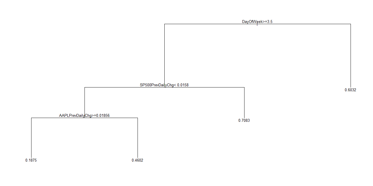
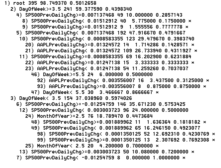
Since 2012
Classification error = 28.3%
Trading days = 395

Since 2013
Classification error = 28.3%
Number of trading days = 145
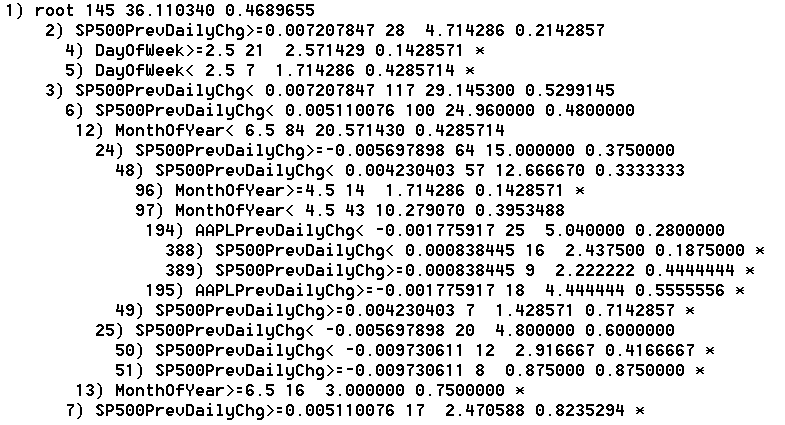
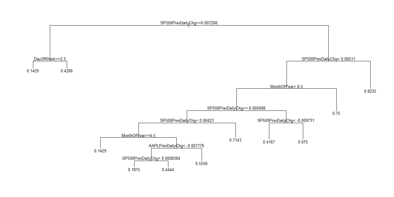
Classification error goes up slightly as the time window narrows. This change makes sense given the reduction in the dataset. The positive trade-off comes in the form of additional classification branches that offer niche trading scenarios. As an example, it is only with the 2013 data that the model is able to discover that July, 2013 was largely an up month for AAPL with 75% of the trading days delivering gains. This branch becomes insignificant with a lot more data, especially when diluted with less definitive Julys (I did not bother to add back the year as an independent variable).
Going back to 2010, the fundamental lesson is that the first two days of the trading week (DayOfTheWeek < 3.5) tend to deliver gains around 60% of the time. However, the final three days of the week basically generate a 50/50 split. The strong tendency of negative ends to the week only show up starting in 2011. For example, if AAPL gains 1.85% or more on a given day, the next day has an 81% chance of being a down day if it is Wednesday, Thursday, or Friday. Friday does not show up as a particular thorn in the side until the time window is reduced to 2012 to 2013. In that tress, node #92 shows a 69% chance of a down day on Friday when Thursday delivers a 0.4% gain or less. These trees do not produce confidence intervals; the classification error rates give a relative sense of reliability. When cherry picking branches of the tree, you must be cognizant of the number (n) of observations used to produce the classification. The more observation, the better in this case. The Apple Trading Model is not particularly complicated. Simplicity is a beautiful thing when trading, especially without computers to manage the trades for you. This simplicity also means that the model can be applied to any stock. It just so happens that I had noticed a pattern in Apple's trading last year and decided to look at the data to confirm my manual observations. The rest is history as they say. The next step is to try to develop a model that gives reasonable predictive power for the magnitude of AAPL's price changes. Stay tuned and be careful out there! Full disclosure: long AAPL shares and puts